Conduction Lens
A calibrated lens on cardiac conduction: what a 12-lead ECG can and cannot resolve about the His-Purkinje system.
01 / the question
Which conduction parameters can an ECG actually determine?
We trained a calibrated neural posterior estimator to answer it, one parameter at a time, at a stated noise floor.
Amortized neural posterior estimation over seven conduction parameters at fixed anatomy, graded with simulation based calibration on the simulator. Synthetic target, no patient data.
Identifiability spectrum: 4 of 7 carry information (2 well resolved, 2 moderate); 3 diffuse
Before trusting any of those numbers, two questions: does it matter, and is the uncertainty honest.
02 / why it matters
The ECG resolves the parameter clinicians actually use
Most of what the ECG resolves is the part clinicians act on.
The interventricular delay, the timing that clinicians program into CRT pacing devices, is the most resolved of the seven parameters.
The tree shape parameters are not resolved at this noise floor, so any single value for them read off an ECG fit is a prior belief, not a measurement.
Anyone fitting conduction models to the ECG can reuse this: the calibrated identifiability recipe, plus the released weights, sweeps, and verification ledger, says which of their own reported parameters are measurements and which are prior beliefs. The same pipeline already runs on the public Strocchi cohort, so a new anatomy is a config change, not a rebuild.
That is the stake. Here is the machine that turns a heart into an ECG, and the ECG back into a distribution over parameters.
03 / the heart and the pipeline
The heart, and the pipeline that inverts it
The anatomy is fixed. Conduction parameters flow through the simulator to a 12-lead ECG; an amortized posterior estimator inverts it. Four steps, no neural-network background needed.
Simulate many hearts
Draw conduction parameters from a prior and run a heart simulator thousands of times to build many parameter to ECG pairs.
Train a network to invert
Train a network to run it backwards: give it an ECG, it returns a distribution over the parameters that could have produced it.
Check its confidence is honest
Grade the network with simulation based calibration, which asks whether its stated uncertainty matches reality, and correct it where it is overconfident.
Report what survives
Report only what the ECG actually narrows, with the noise floor stated, and flag plainly what it cannot resolve.
the forward model, in two examples
Activation map
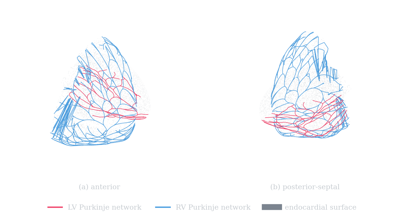
local activation time (ms)LV and RV fractal Purkinje networks (the real trees that seed this activation: 3178 nodes, 253 Purkinje-muscle junctions).
The myocardial surface coloured by activation time, with the Purkinje network that produced it. An example of the forward model, not evidence for the finding.
Forward 12-lead ECG
synthetic target at the reference parametersThe forward-model 12-lead pseudo-ECG at the reference conduction parameters. Amplitudes are arbitrary units scaled to a stated mV operating point. This is not a comparison against a real ECG.
Run that pipeline across the prior and read off, parameter by parameter, how much the ECG actually narrows.
04 / the finding, in full
Four of seven parameters carry information
At the waveform floor (sigma 0.025 mV per sample per lead) the ordering is clear. Interventricular delay (contraction about 0.15) and myocardial velocity (about 0.35) are well constrained; RV initial extent (about 0.63) and conduction velocity (about 0.67) are moderate; LV extent, branch angle and branch repulsivity stay diffuse (about 1.0 to 1.2), no tighter than the prior.
Identifiability spectrum: 4 of 7 carry information (2 well resolved, 2 moderate); 3 diffuse
at a noise floor of 0.025 mV
LV-RV interventricular delay
The ECG narrows it to about 10 to 23 ms (90% interval), keeping only 15% of the prior width.
branch angle
The posterior still spans 0.097 to 0.316 rad, keeping 121% of the prior. Any single value read off an ECG fit for it is a prior belief, not a measurement.
Contraction = posterior std / prior std, per parameter. Lower is better resolved. Bars show the posterior 90% interval inside the prior range; the amber tick is the synthetic truth. Resolved, moderate and diffuse are stated at the noise floor above, not in the absolute.
05 / is the uncertainty honest?
Calibrated, so the intervals mean what they say
An identifiability claim is only as good as its calibration. The raw posterior was overconfident; per-parameter conformal recalibration flattens the simulation based calibration ranks and brings the joint coverage to the diagonal. Toggle before and after.
SBC KS p-values (per parameter)
SBC rank-uniformity test per parameter, p above 0.05 (green) does not reject calibration.
Joint coverage after conformal (TARP)
Expected-coverage (TARP) curve: nominal credibility level (x) versus empirical coverage (y). On the dashed diagonal is calibrated; below it is overconfident. Joint ATC -0.057 before conformal to +0.007 after: the recalibrated joint is brought to approximate coverage (a negative ATC is overconfident; near zero is calibrated).
Calibrated marginals still hide how parameters trade off against each other. One pair shows it clearly.
06 / the correlated pair
Correlated, but still identifiable
Interventricular delay and RV initial extent trade off against each other: the ECG constrains their combination more tightly than either alone, while leaving each one looser. That is correlation, not a failure to resolve.
Reading the plot
- Diagonal: each parameter's marginal posterior, coloured by how well the ECG resolves it.
- Lower cells: pairwise samples. A tilted cloud means the pair is correlated.
- The amber cell: the dIV to L0_RV pair, the strongest correlation where both parameters are still individually identifiable.
- Upper cells: correlation strength between parameters.
Why it matters
A single best fit would hide this. The calibrated posterior shows the ECG measures a combination faithfully while leaving each ingredient looser, the kind of finding a point estimate cannot express.
07 / limitations
Limitations
- A simulated ECG. Not a recording from a patient.
- One geometry. Not a cohort.
- A pseudo-ECG in an unbounded homogeneous volume conductor. Amplitudes are arbitrary units scaled to a stated mV operating point. Absolute calibration is not claimed.
- A local Jacobian. Not a global sensitivity analysis.
- No patient data anywhere.
08 / the pipeline generalizes
The pipeline generalizes
The same steps run on multiple public anatomies. This is a claim about the method, not a second result.
LV and RV fractal Purkinje networks (the real trees that seed this activation: 4249 nodes, 338 Purkinje-muscle junctions).
Figure 2. Strocchi heart 01: grown LV / RV Purkinje network, 200 / 138 Purkinje-muscle junctions.
LV and RV fractal Purkinje networks (the real trees that seed this activation: 8684 nodes, 695 Purkinje-muscle junctions).
Figure 3. Strocchi heart 02: grown LV / RV Purkinje network, 394 / 301 Purkinje-muscle junctions.
The pipeline ingests public CC-BY-4.0 four-chamber meshes (Strocchi et al., PLoS ONE 2020), derives each endocardium from the mesh's own universal ventricular coordinates, grows a Purkinje network, places electrodes from the heart's own axes, and synthesizes a pseudo-ECG. This demonstrates that the method generalizes to real anatomy. No identifiability result is claimed on any of these hearts (crtdemo's PMJ counts are 87 and 166 for reference).
Everything above is a static export from a named run. Here is how to reproduce it.
09 / reproduce and read the paper
Everything you need to run it yourself
The finding is a static export from a named run. The code, the weights, and the environment are open.
The paper
IEEE / Zenodo manuscriptThe full write-up: methods, the calibrated identifiability spectrum, calibration, and the honest limitations, as a self-contained IEEE-format paper.
Read the paper (Zenodo)Verification ledger
every claim, checkedThe record of what was claimed, what was checked, and what was retracted. The corrections above are drawn from it.
docs/verification-ledger.mdWeights and container
the trained network and its environmentThe trained posterior estimator and a container image that pins the full environment, so a run reproduces bit for bit.
github.com/ricardogr07/ecg-purkinje-npeCode license
Apache-2.0All code in this project is released under Apache-2.0. Use it, fork it, build on it.
Data license
Strocchi CC-BY-4.0The Strocchi biventricular mesh cohort is used under CC-BY-4.0, with attribution to the original authors.